In Mathematics, the Bisection Method is a straightforward method used to find numerical solutions of an equation with one unknown variable.
Index
Definition
This method is a root-finding method that applies to any continuous functions with two known values of opposite signs. It is a very simple but cumbersome method.
The interval defined by these two values is bisected and a sub-interval in which the function changes sign is selected. This sub-interval must contain the root. These two steps are repeatedly executed until the root is in the form of the required precision level.
This method is also called as interval halving method, the binary method, or the dichotomy method.
The Method: Explained
Let \(f\) be a continuous function defined on an interval \([a, b]\) where \(f(a)\) and \(f(b)\) have opposite signs. Bisection method is applicable for solving the equation \(f(x) = 0\) for a real variable \(x\).
At each step, the interval is divided into two parts/halves by computing the midpoint, \(c = \frac{(a+b)}{2}\), and the value of \(f(c)\) at that point. Unless the root is \(c\), there are two possibilities:
- \(f(a)\) and \(f(c)\) have opposite signs and bracket a root,
- \(f(c)\) and \(f(b)\) have opposite signs and bracket a root.
One of the sub-intervals is chosen as the new interval to be used in the next step. This process is carried out again and again until the interval is sufficiently small.
If \(f(a)\) and \(f(c)\) have opposite signs, then the value of \(b\) is replaced by \(c\).
If \(f(b)\) and \(f(c)\) have opposite signs, then the value of \(a\) is replaced by \(c\).
In the case that \(f(c) = 0, c\) will be taken as the solution and the process stops.
Bisection Method Algorithm
The algorithm for the bisection method is as below:
INPUT: Function \(f\), endpoint values \(a, b\), tolerance \(TOL\), maximum iterations \(NMAX\).
OUTPUT: value that differs from the root of \(f(x) = 0\) by less than \(TOL\).
N ← 1
while N <= NMAX do
    C ← (a + b)/2
    if f(c) = 0 or (b - a)/2 < TOL then
        Output(c)
        stop
    end if
    N ← N + 1
    if sign(f(c)) = sign(f(a)) then
        a ← c
    else
        b ← c
end while
Output(“Method failed.”)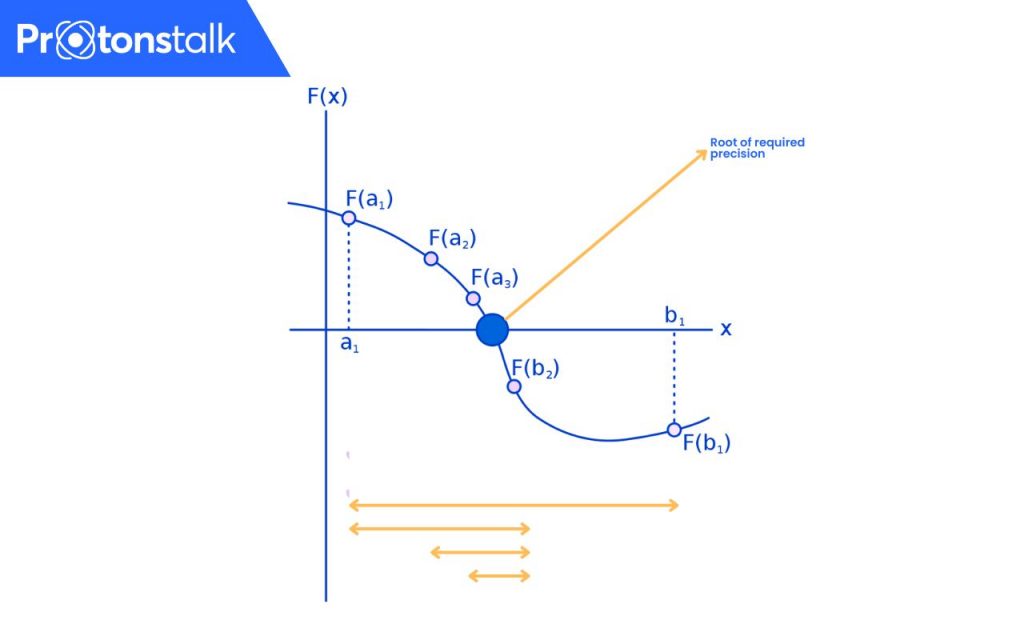
Advantages & Disadvantages of Bisection Method
| Advantages | Disadvantages |
| Convergence is guaranteed. | A slow, linear rate of convergence. |
| The error can be controlled. | Cannot find the root of some equations. |
| Simple and easy to program. | If one of the guesses is closer to the root, it will still take a larger number of iterations |
Solved Examples
Here, we have bisection method example problems with solution.
Question. Determine the root of the equation, \(f(x) = x^3 – x – 2\) for \(x ∈ [1, 2]\).
Solution. Given,
\(f(x) = x^3 – x – 2\) for \(x ∈ [1, 2]\)
Take, \(a = 1, b = 2\)
\(f(1) = 1^3 – 1 – 2 = -2\)
\(f(2) = 2^3 – 2 – 2 = +4\)
As the function is continuous, a root must lie within [1, 2].
1st Iteration:
\(a_1 = 1, b_1= 2\),
\(c_1= \frac{2 + 1}{2} = 1.5\)
Hence, the function value at midpoint is,
\(f(c_1) = (1.5)^3 – (1.5) – 2 = -0.125\)
As \(f(c)\) gives a negative value, the value of \(a\) is replaced by \(c\).
The iterations are concisely summarized into a table below:
| Iteration | \(a_n\) | \(b_n\) | \(c_n\) | \(f(c_n)\) |
| 1 | 1 | 2 | 1.5 | −0.125 |
| 2 | 1.5 | 2 | 1.75 | 1.6093750 |
| 3 | 1.5 | 1.75 | 1.625 | 0.6660156 |
| 4 | 1.5 | 1.625 | 1.5625 | 0.2521973 |
| 5 | 1.5 | 1.5625 | 1.5312500 | 0.0591125 |
| 6 | 1.5 | 1.5312500 | 1.5156250 | −0.0340538 |
| 7 | 1.5156250 | 1.5312500 | 1.5234375 | 0.0122504 |
| 8 | 1.5156250 | 1.5234375 | 1.5195313 | −0.0109712 |
| 9 | 1.5195313 | 1.5234375 | 1.5214844 | 0.0006222 |
| 10 | 1.5195313 | 1.5214844 | 1.5205078 | −0.0051789 |
| 11 | 1.5205078 | 1.5214844 | 1.5209961 | −0.0022794 |
| 12 | 1.5209961 | 1.5214844 | 1.5212402 | −0.0008289 |
| 13 | 1.5212402 | 1.5214844 | 1.5213623 | −0.0001034 |
| 14 | 1.5213623 | 1.5214844 | 1.5214233 | 0.0002594 |
| 15 | 1.5213623 | 1.5214233 | 1.5213928 | 0.0000780 |
From the above table, it can be pointed out that, after 13 iterations, it becomes apparent that the function converges to 1.521, which is concluded as the root of the polynomial.
Related Articles
1. Newton Raphson Method
2. Secant Method
FAQs
Following are the applications of the bisection method:
– Applied to LiNC/LiCN molecular system to locate periodic orbits,
– To find roots of continuous functions.
The bisection method is slower than the Newton Raphson method as the former method has a higher convergence rate compared to the latter.